Data Labelling¶

The simplest approach to supvervised financial machine learning is to aim to predict the price of an instrument at some fixed horison. But due to the nature of the data, this goal is practically unachievable. Another approach is to focus on the classification problem, i.e. predict discretized returns. Classification problem with finite set of possible labels has a greater chan to obtain predictive power than regression problem where the pool of outcome is virtually infinite.

This module implemented both the commonly used as well as a couple of interesting techniques for labeling financial data. The vast majority of our users make use of the following labeling schemes (in a classification setting):

Raw Returns

Fixed Horizon

Triple-Barrier and Meta-labeling

Trend Scanning

Raw Returns¶

Labeling data by raw returns is the most simple and basic method of labeling financial data for machine learning. Raw returns can be calculated either on a simple or logarithmic basis. Using returns rather than prices is usually preferred for financial time series data because returns are usually stationary, unlike prices. This means that returns across different assets, or the same asset at different times, can be directly compared with each other. The same cannot be said of price differences, since the magnitude of the price change is highly dependent on the starting price, which varies with time.

The simple return for an observation with price \(p_t\) at time \(t\) relative to its price at time \(t-1\) is as follows:

\[r_t = \frac{p_{t}}{p_{t-1}} - 1\]

And the logarithmic return is:

\[r_t = log(p_t) - log(p_{t-1})\]

The label \(L_t\) is simply equal to \(r_t\), or to the sign of \(r_t\), if binary labeling is desired.

\[\begin{split}\begin{equation} \begin{split} L_{t} = \begin{cases} -1 &\ \text{if} \ \ r_t < 0\\ 0 &\ \text{if} \ \ r_t = 0\\ 1 &\ \text{if} \ \ r_t > 0 \end{cases} \end{split} \end{equation}\end{split}\]

If desired, the user can specify a resampling period to apply to the price data prior to calculating returns. The user can also lag the returns to make them forward-looking.

The following shows the distribution of logarithmic daily returns on Microsoft stock during the time period between January 2010 and May 2020.

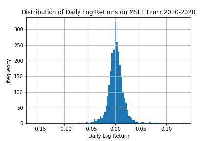
raw returns image — Distribution of logarithmic returns on MSFT.¶

Implementation¶

Raw Returns Labeling Method

Most basic form of labeling based on raw return of each observation relative to its previous value.

mlfinpy.labeling.raw_return.raw_return(prices: Series | DataFrame, binary: bool = False, logarithmic: bool = False, resample_by: str | None = None, lag: bool = True) → Series | DataFrame[source]¶

Raw returns labeling method.

This is the most basic and ubiquitous labeling method used as a precursor to almost any kind of financial data analysis or machine learning. User can specify simple or logarithmic returns, numerical or binary labels, a resample period, and whether returns are lagged to be forward looking.

Parameters¶

pricespd.Series or pd.DataFrame: Time-indexed price data on stocks with which to calculate return.
binarybool: If False, will return numerical returns. If True, will return the sign of the raw return.
logarithmicbool: If False, will calculate simple returns. If True, will calculate logarithmic returns.
resample_bystr or None: If not None, the resampling period for price data prior to calculating returns. ‘B’ = per business day, ‘W’ = week, ‘M’ = month, etc. Will take the last observation for each period. For full details see here.
lagbool: If True, returns will be lagged to make them forward-looking.

Returns¶

pd.Series or pd.DataFrame: Raw returns on market data. User can specify whether returns will be based on simple or logarithmic return, and whether the output will be numerical or categorical.

Example¶

Below is an example on how to use the raw returns labeling method.

import pandas as pd
from mlfinpy.labeling import raw_return

# Import price data
data = pd.read_csv('../Sample-Data/stock_prices.csv', index_col='Date', parse_dates=True)

# Create labels numerically based on simple returns
returns = raw_returns(prices=data, lag=True)

# Create labels categorically based on logarithmic returns
returns = raw_returns(prices=data, binary=True, logarithmic=True, lag=True)

# Create labels categorically on weekly data with forward looking log returns.
returns = raw_returns(prices=data, binary=True, logarithmic=True, resample_by='W', lag=True)

Fixed Time Horizon¶

Fixed horizon labels is a classification labeling technique used in the following paper: Dixon, M., Klabjan, D. and Bang, J., 2016. Classification-based Financial Markets Prediction using Deep Neural Networks.

Fixed time horizon is a common method used in labeling financial data, usually applied on time bars. The rate of return relative to \(t_0\) over time horizon \(h\), assuming that returns are lagged, is calculated as follows (M.L. de Prado, Advances in Financial Machine Learning, 2018):

\[r_{t0,t1} = \frac{p_{t1}}{p_{t0}} - 1\]

Where \(t_1\) is the time bar index after a fixed horizon has passed, and \(p_{t0}, p_{t1}\) are prices at times \(t_0, t_1\). This method assigns a label based on comparison of rate of return to a threshold \(\tau\)

\[\begin{split}\begin{equation} \begin{split} L_{t0, t1} = \begin{cases} -1 &\ \text{if} \ \ r_{t0, t1} < -\tau\\ 0 &\ \text{if} \ \ -\tau \leq r_{t0, t1} \leq \tau\\ 1 &\ \text{if} \ \ r_{t0, t1} > \tau \end{cases} \end{split} \end{equation}\end{split}\]

To avoid overlapping return windows, rather than specifying \(h\), the user is given the option of resampling the returns to get the desired return period. Possible inputs for the resample period can be found here.. Optionally, returns can be standardized by scaling by the mean and standard deviation of a rolling window. If threshold is a pd.Series, threshold.index and prices.index must match; otherwise labels will fail to be returned. If resampling is used, the threshold must match the index of prices after resampling. This is to avoid the user being forced to manually fill in thresholds.

The following shows the distribution of labels for standardized returns on closing prices of SPY in the time period from Jan 2008 to July 2016 using a 20-day rolling window for the standard deviation.

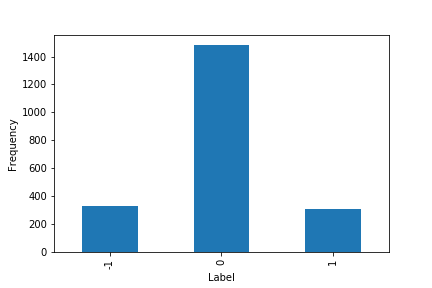
fixed horizon example — Distribution of labels on standardized returns on closing prices of SPY.¶

Though time bars are the most common format for financial data, there can be potential problems with over-reliance on time bars. Time bars exhibit high seasonality, as trading behavior may be quite different at the open or close versus midday; thus it will not be informative to apply the same threshold on a non-uniform distribution. Solutions include applying the fixed horizon method to tick or volume bars instead of time bars, using data sampled at the same time every day (e.g. closing prices) or inputting a dynamic threshold as a pd.Series corresponding to the timestamps in the dataset. However, the fixed horizon method will always fail to capture information about the path of the prices [Lopez de Prado, 2018].

Tip

Underlying Literature

The following sources describe this method in more detail:

Advances in Financial Machine Learning, Chapter 3.2 by Marcos Lopez de Prado (p. 43-44).
Machine Learning for Asset Managers, Chapter 5.2 by Marcos Lopez de Prado (p. 65-66).

Implementation¶

Fixed-Time-Horizon Labeling Method

The article “Classification-based Financial Markets Prediction using Deep Neural Networks” by Dixon et al. (2016) describes how labeling data this way can be used in training deep neural networks to predict price movements.

Fixed-Time Horizon Labeling Method.

This method is originally described in the book Advances in Financial Machine Learning, Chapter 3.2, p.43-44.

Returns 1 if return is greater than the threshold, -1 if less, and 0 if in between. If no threshold is provided then it will simply take the sign of the return.

Parameters¶

pricespd.Series or pd.DataFrame: Time-indexed stock prices used to calculate returns.
thresholdfloat or pd.Series, optional: When the absolute value of return exceeds the threshold, the observation is labeled with 1 or -1, depending on the sign of the return. If return is less, it’s labeled as 0. Can be dynamic if threshold is inputted as a pd.Series, and threshold.index must match prices.index. If resampling is used, the index of threshold must match the index of prices after resampling. If threshold is negative, then the directionality of the labels will be reversed. If no threshold is provided, it is assumed to be 0 and the sign of the return is returned.
resample_bystr, optional: If not None, the resampling period for price data prior to calculating returns. ‘B’ = per business day, ‘W’ = week, ‘M’ = month, etc. Will take the last observation for each period. For full details see here.
lagbool, optional: If True, returns will be lagged to make them forward-looking.
standardizedbool, optional: Whether returns are scaled by mean and standard deviation.
windowint, optional: If standardized is True, the rolling window period for calculating the mean and standard deviation of returns.

Returns¶

pd.Series or pd.DataFrame: -1, 0, or 1 denoting whether the return for each observation is less/between/greater than the threshold at each corresponding time index. First or last row will be NaN, depending on lag.

Example¶

Below is an example on how to use the Fixed Horizon labeling technique on real data.

import pandas as pd
import numpy as np

from mlfinpy.labeling import fixed_time_horizon

# Import price data.
data = pd.read_csv('../Sample-Data/stock_prices.csv', index_col='Date', parse_dates=True)
custom_threshold = pd.Series(np.random.random(len(data)), index = data.index)

# Create labels.
labels = fixed_time_horizon(prices=data, threshold=0.01, lag=True)

# Create labels with a dynamic threshold.
labels = fixed_time_horizon(prices=data, threshold=custom_threshold, lag=True)

# Create labels with standardization.
labels = fixed_time_horizon(prices=data, threshold=1, lag=True, standardized=True, window=5)

# Create labels after resampling weekly with standardization.
labels = fixed_time_horizon(prices=data, threshold=1, resample_by='W', lag=True,
                            standardized=True, window=4)

Triple-Barrier and Meta-Labelling¶

The primary labeling method used in financial academia is the fixed-time horizon method. While ubiquitous, this method has many faults which are remedied by the triple-barrier method discussed below. The triple-barrier method can be extended to incorporate meta-labeling which will also be demonstrated and discussed below.

Triple-Barrier Method¶

The idea behind the triple-barrier method is that we have three barriers: an upper barrier, a lower barrier, and a vertical barrier. The upper barrier represents the threshold an observation’s return needs to reach in order to be considered a buying opportunity (a label of 1), the lower barrier represents the threshold an observation’s return needs to reach in order to be considered a selling opportunity (a label of -1), and the vertical barrier represents the amount of time an observation has to reach its given return in either direction before it is given a label of 0. This concept can be better understood visually and is shown in the figure below taken from Advances in Financial Machine Learning (reference):

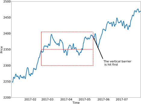
One of the major faults with the fixed-time horizon method is that observations are given a label with respect to a certain threshold after a fixed interval regardless of their respective volatilities. In other words, the expected returns of every observation are treated equally regardless of the associated risk. The triple-barrier method tackles this issue by dynamically setting the upper and lower barriers for each observation based on their given volatilities.

Meta-Labeling¶

Advances in Financial Machine Learning, Chapter 3, page 50. Reads:

“Suppose that you have a model for setting the side of the bet (long or short). You just need to learn the size of that bet, which includes the possibility of no bet at all (zero size). This is a situation that practitioners face regularly. We often know whether we want to buy or sell a product, and the only remaining question is how much money we should risk in such a bet. We do not want the ML algorithm to learn the side, just to tell us what is the appropriate size. At this point, it probably does not surprise you to hear that no book or paper has so far discussed this common problem. Thankfully, that misery ends here.””

I call this problem meta-labeling because we want to build a secondary ML model that learns how to use a primary exogenous model.

The ML algorithm will be trained to decide whether to take the bet or pass, a purely binary prediction. When the predicted label is 1, we can use the probability of this secondary prediction to derive the size of the bet, where the side (sign) of the position has been set by the primary model.

Meta-Labeling User Guide¶

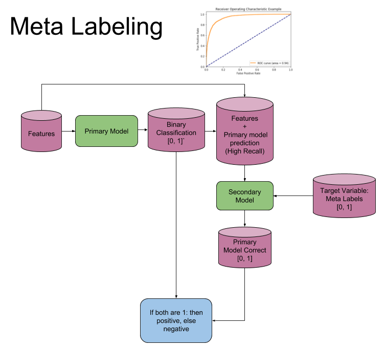
Binary classification problems present a trade-off between type-I errors (false positives) and type-II errors (false negatives). In general, increasing the true positive rate of a binary classifier will tend to increase its false positive rate. The receiver operating characteristic (ROC) curve of a binary classifier measures the cost of increasing the true positive rate, in terms of accepting higher false positive rates.

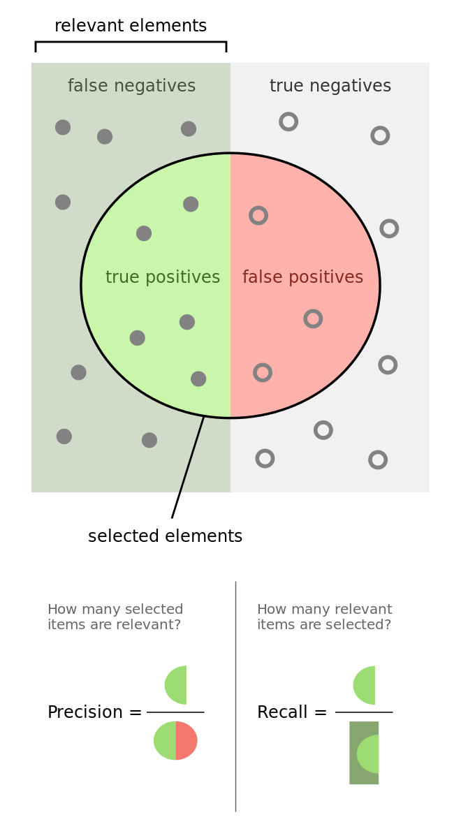
The image illustrates the so-called “confusion matrix.” On a set of observations, there are items that exhibit a condition (positives, left rectangle), and items that do not exhibit a condition (negative, right rectangle). A binary classifier predicts that some items exhibit the condition (ellipse), where the TP area contains the true positives and the TN area contains the true negatives. This leads to two kinds of errors: false positives (FP) and false negatives (FN). “Precision” is the ratio between the TP area and the area in the ellipse. “Recall” is the ratio between the TP area and the area in the left rectangle. This notion of recall (aka true positive rate) is in the context of classification problems, the analogous to “power” in the context of hypothesis testing. “Accuracy” is the sum of the TP and TN areas divided by the overall set of items (square). In general, decreasing the FP area comes at a cost of increasing the FN area, because higher precision typically means fewer calls, hence lower recall. Still, there is some combination of precision and recall that maximizes the overall efficiency of the classifier. The F1-score measures the efficiency of a classifier as the harmonic average between precision and recall.

Meta-labeling is particularly helpful when you want to achieve higher F1-scores. First, we build a model that achieves high recall, even if the precision is not particularly high. Second, we correct for the low precision by applying meta-labeling to the positives predicted by the primary model.

Meta-labeling will increase your F1-score by filtering out the false positives, where the majority of positives have already been identified by the primary model. Stated differently, the role of the secondary ML algorithm is to determine whether a positive from the primary (exogenous) model is true or false. It is not its purpose to come up with a betting opportunity. Its purpose is to determine whether we should act or pass on the opportunity that has been presented.

Meta-labeling is a very powerful tool to have in your arsenal, for four additional reasons:

First, ML algorithms are often criticized as black boxes. Meta-labeling allows you to build an ML system on top of a white box (like a fundamental model founded on economic theory). This ability to transform a fundamental model into an ML model should make meta-labeling particularly useful to “quantamental” firms.

Second, the effects of overfitting are limited when you apply metalabeling, because ML will not decide the side of your bet, only the size.

Third, by decoupling the side prediction from the size prediction, meta-labeling enables sophisticated strategy structures. For instance, consider that the features driving a rally may differ from the features driving a sell-off. In that case, you may want to develop an ML strategy exclusively for long positions, based on the buy recommendations of a primary model, and an ML strategy exclusively for short positions, based on the sell recommendations of an entirely different primary model.

Fourth, achieving high accuracy on small bets and low accuracy on large bets will ruin you. As important as identifying good opportunities is to size them properly, so it makes sense to develop an ML algorithm solely focused on getting that critical decision (sizing) right. We will retake this fourth point in Chapter 10. In my experience, meta-labeling ML models can deliver more robust and reliable outcomes than standard labeling models.

Model Architecture¶

The following image explains the model architecture. The first step is to train a primary model (binary classification). Second a threshold level is determined at which the primary model has a high recall, in the coded example you will find that 0.30 is a good threshold, ROC curves could be used to help determine a good level. Third the features from the first model are concatenated with the predictions from the first model, into a new feature set for the secondary model. Meta Labels are used as the target variable in the second model. Now fit the second model. Fourth the prediction from the secondary model is combined with the prediction from the primary model and only where both are true, is your final prediction true. I.e. if your primary model predicts a 3 and your secondary model says you have a high probability of the primary model being correct, is your final prediction a 3, else not 3.

Implementation¶

The following functions are used for the triple-barrier method which works in tandem with meta-labeling.

mlfinpy.labeling.labeling.add_vertical_barrier(t_events, close, num_days=0, num_hours=0, num_minutes=0, num_seconds=0)[source]¶

Adding a Vertical Barrier

For each index in t_events, it finds the timestamp of the next price bar at or immediately after a number of days num_days. This vertical barrier can be passed as an optional argument t1 in get_events.

This function creates a series that has all the timestamps of when the vertical barrier would be reached.

Parameters¶

t_eventspd.Series: Series of events timestamps from the filters e.g. Cusum filter, Z-score filter.
closepd.Series: Close prices series.
num_daysint, optional: Number of days to add for vertical barrier.
num_hoursint, optional: Number of hours to add for vertical barrier.
num_minutesint, optional: Number of minutes to add for vertical barrier.
num_secondsint, optional: Number of seconds to add for vertical barrier.

Returns¶

verticle_barrierspd.Series: Timestamps of vertical barriers.

Notes¶

Advances in Financial Machine Learning, Snippet 3.4, page 49.

mlfinpy.labeling.labeling.get_events(close: Series, t_events: Series, pt_sl: List[float], target: Series, min_ret: float, num_threads: int, vertical_barrier_times: Series | bool = False, side_prediction: Series | None = None, verbose: bool = True) → DataFrame[source]¶

Advances in Financial Machine Learning, Snippet 3.6 page 50.

Getting the Time of the First Touch, with Meta Labels

This function is orchestrator to meta-label the data, in conjunction with the Triple Barrier Method.

Parameters¶

closepd.Series: Close prices
t_eventspd.Series: of t_events. These are timestamps that will seed every triple barrier. These are the timestamps selected by the sampling procedures discussed in Chapter 2, Section 2.5. Eg: CUSUM Filter
pt_slList[float]: Element 0, indicates the profit taking level; Element 1 is stop loss level. A non-negative float that sets the width of the two barriers. A 0 value means that the respective horizontal barrier (profit taking and/or stop loss) will be disabled.
targetpd.Series: of values that are used (in conjunction with pt_sl) to determine the width of the barrier. In this program this is daily volatility series.
min_retfloat: The minimum target return required for running a triple barrier search.
num_threadsint: The number of threads concurrently used by the function.
vertical_barrier_timesUnion[pd.Series, bool]: A pandas series with the timestamps of the vertical barriers. We pass a False when we want to disable vertical barriers.
side_predictionOptional[pd.Series]: Side of the bet (long/short) as decided by the primary model
verbosebool: Flag to report progress on asynch jobs

Returns¶

eventspd.DataFrame: Dataframe of first touch events with meta-labels. - events.index is event’s starttime - events[‘t1’] is event’s endtime - events[‘trgt’] is event’s target - events[‘side’] (optional) implies the algo’s position side - events[‘pt’] is profit taking multiple - events[‘sl’] is stop loss multiple

mlfinpy.labeling.labeling.get_bins(triple_barrier_events: DataFrame, close: Series) → DataFrame[source]¶

Labeling for Side & Size with Meta Labels

Compute event’s outcome (including side information, if provided). events is a DataFrame where:

Now the possible values for labels in out[‘bin’] are {0,1}, as opposed to whether to take the bet or pass, a purely binary prediction. When the predicted label the previous feasible values {−1,0,1}. The ML algorithm will be trained to decide is 1, we can use the probability of this secondary prediction to derive the size of the bet, where the side (sign) of the position has been set by the primary model.

Parameters¶

triple_barrier_eventspd.DataFrame: DataFrame returned by ‘get_events’ with columns: - index: event starttime - vertical_barriers: event endtime - trgt: event target - side (optional): position side Case 1: (‘side’ not in events): bin in (-1,1) <-label by price action. Case 2: (‘side’ in events): bin in (0,1) <-label by pnl (meta-labeling).
closepd.Series: Close prices series.

Returns¶

out_dfpd.DataFrame: Meta-labeled events.

Notes¶

Advances in Financial Machine Learning, Snippet 3.7, page 51.

mlfinpy.labeling.labeling.drop_labels(events: DataFrame, min_pct: float = 0.05) → DataFrame[source]¶

This function recursively eliminates rare observations.

Parameters¶

eventspd.DataFrame: Events.
min_pctfloat, optional: A fraction used to decide if the observation occurs less than that fraction. Defaults to .05.

Returns¶

pd.DataFrame: Events.

Notes¶

Advances in Financial Machine Learning, Snippet 3.8 page 54.

Example¶

Suppose we use a mean-reverting strategy as our primary model, giving each observation a label of -1 or 1. We can then use meta-labeling to act as a filter for the bets of our primary model.

Assuming we have a pandas series with the timestamps of our observations and their respective labels given by the primary model, the process to generate meta-labels goes as follows.

import numpy as np
import pandas as pd
import mlfinpy as ml

# Read in data
data = pd.read_csv('FILE_PATH')

# Compute daily volatility
daily_vol = ml.util.get_daily_vol(close=data['close'], lookback=50)

# Apply Symmetric CUSUM Filter and get timestamps for events
# Note: Only the CUSUM filter needs a point estimate for volatility
cusum_events = ml.filters.cusum_filter(data['close'],
                                       threshold=daily_vol['2011-09-01':'2018-01-01'].mean())

# Compute vertical barrier
vertical_barriers = ml.labeling.add_vertical_barrier(t_events=cusum_events,
                                                     close=data['close'],
                                                     num_days=1)

Once we have computed the daily volatility along with our vertical time barriers and have downsampled our series using the CUSUM filter, we can use the triple-barrier method to compute our meta-labels by passing in the side predicted by the primary model.

pt_sl = [1, 2]
min_ret = 0.005
triple_barrier_events = ml.labeling.get_events(close=data['close'],
                                               t_events=cusum_events,
                                               pt_sl=pt_sl,
                                               target=daily_vol,
                                               min_ret=min_ret,
                                               num_threads=3,
                                               vertical_barrier_times=vertical_barriers,
                                               side_prediction=data['side'])

As can be seen above, we have scaled our lower barrier and set our minimum return to 0.005.

Meta-labels can then be computed using the time that each observation touched its respective barrier.

meta_labels = ml.labeling.get_bins(triple_barrier_events, data['close'])

Trend Scanning¶

Trend Scanning is both a classification and regression labeling technique introduced by Marcos Lopez de Prado in the following lecture slides: Advances in Financial Machine Learning, Lecture 3/10, and again in his text book Machine Learning for Asset Managers.

For some trading algorithms, the researcher may not want to explicitly set a fixed profit / stop loss level, but rather detect overall trend direction and sit in a position until the trend changes. For example, market timing strategy which holds ETFs except during volatile periods. Trend scanning labels are designed to solve this type of problems.

This algorithm is also useful for defining market regimes between downtrend, no-trend, and uptrend.

The idea of trend-scanning labels are to fit multiple regressions from time t to t + L (L is a maximum look-forward window) and select the one which yields maximum t-value for the slope coefficient, for a specific observation.

Tip

Classification: By taking the sign of t-value for a given observation we can set {-1, 1} labels to define the trends as either downward or upward.
Classification: By adding a minimum t-value threshold you can generate {-1, 0, 1} labels for downward, no-trend, upward.
The t-values can be used as sample weights in classification problems.
Regression: The t-values can be used in a regression setting to determine the magnitude of the trend.

The output of this algorithm is a DataFrame with t1 (time stamp for the farthest observation), t-value, returns for the trend, and bin.

Implementation¶

Implementation of Trend-Scanning labels described in Advances in Financial Machine Learning: Lecture 3/10

mlfinpy.labeling.trend_scanning.trend_scanning_labels(price_series: Series, t_events: list | None = None, look_forward_window: int = 20, min_sample_length: int = 5, step: int = 1) → DataFrame[source]¶

Trend scanning is both a classification and regression labeling technique.

That can be used in the following ways:

Classification: By taking the sign of t-value for a given observation we can set {-1, 1} labels to define the trends as either downward or upward.
Classification: By adding a minimum t-value threshold you can generate {-1, 0, 1} labels for downward, no-trend, upward.
The t-values can be used as sample weights in classification problems.
Regression: The t-values can be used in a regression setting to determine the magnitude of the trend.

The output of this algorithm is a DataFrame with t1 (time stamp for the farthest observation), t-value, returns for the trend, and bin.

Parameters¶

price_seriespd.Series: Close prices used to label the data set.
t_eventsOptional[list]: Filtered events, array of pd.Timestamps.
look_forward_windowint: Maximum look forward window used to get the trend value.
min_sample_lengthint: Minimum sample length used to fit regression.
stepint: Optimal t-value index is searched every ‘step’ indices.

Returns¶

pd.DataFrame: Consists of t1, t-value, ret, bin (label information). t1 - label endtime, tvalue, ret - price change %, bin - label value based on price change sign

Example¶

import numpy as np
import pandas as pd

from mlfinpy.labeling import trend_scanning_labels

eem_close = pd.read_csv('./test_data/stock_prices.csv', index_col=0, parse_dates=[0])
# In 2008, EEM had some clear trends
eem_close = eem_close['EEM'].loc[pd.Timestamp(2008, 4, 1):pd.Timestamp(2008, 10, 1)]


t_events = eem_close.index # Get indexes that we want to label
# We look at a maximum of the next 20 days to define the trend, however we fit regression on samples with length >= 10
tr_scan_labels = trend_scanning_labels(eem_close, t_events, look_forward_window=20, min_sample_length=10)